How To Link A Cell To Another Sheet In Excel - An Ultimate Guide
Learn how to link a cell to another sheet in excel with this comprehensive guide to cell linking, mastering data management with ease.
Author:Tyreece BauerReviewer:Gordon DickersonDec 07, 2023116.1K Shares1.6M Views
In the dynamic world of data analysis, spreadsheets have become indispensable tools for managing and manipulating information. Among the many powerful features of Excel, cell linking stands out as a crucial technique for streamlining workflows and enhancing data management. This comprehensive guide delves intohow to link a cell to another sheet in excel, empowering you to seamlessly connect data and achieve greater efficiency in your spreadsheet tasks. Imagine a scenario where you're working on an extensive Excel workbook, tracking sales figures for various departments and regions. As you delve into individual sales reports, you realize the need to consolidate data from different sheets to analyze overall sales performance. This is where cell linking comes into play.
Cell linking, as the name suggests, establishes a connection between cells in different sheets of an Excel workbook. This connection allows you to reference data from one sheet in another, ensuring that any changes made in the source sheet are automatically reflected in the linked cells.
Linking Cells Using Formulas
The formula-based method of cell linking is a fundamental technique for establishing connections between cells in different Excel sheets. This method utilizes formulas to create dynamic links that automatically update whenever the source data changes.
Understanding Excel Link Formula
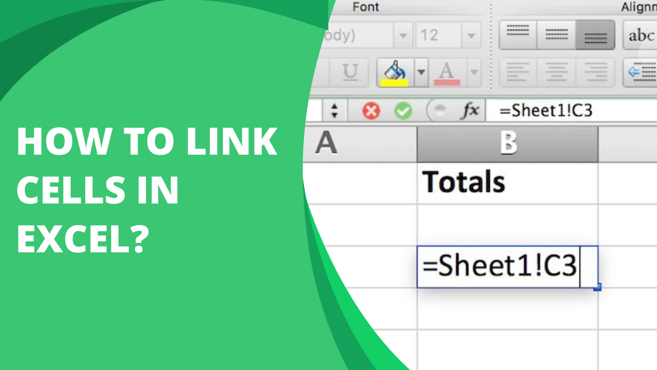
At the heart of formula-based cell linking lies the excel linking formula itself. The syntax of the formula is straightforward and follows a specific structure:
=SheetName!CellReference
Here's a breakdown of the formula components:
- Equal Sign (=) -The equal sign initiates the formula and indicates that a calculation will be performed.
- SheetName -This represents the name of the sheet containing the cell you want to link to. Enclose the sheet name in single quotation marks (').
- CellReference -This specifies the exact cell you want to link to. Use the standard cell reference format, such as A1, B2, or C3.
For instance, to link cell A1 in Sheet1 to cell B2 in Sheet2, you would enter the following formula in cell A1 of Sheet1:
=Sheet2!B2
Instructions
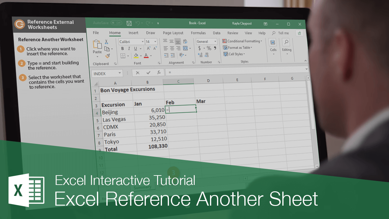
Creating a cell link using a formula is a simple process that can be accomplished in a few steps:
- Select the Destination Cell -Identify the cell in the destination sheet where you want to display the linked data.
- Activate the Formula Bar -Click on the selected cell to activate the formula bar.
- Enter the Formula -Type the formula following the syntax described earlier. For example, if you want to link to cell B2 in Sheet2, enter =Sheet2!B2.
- Press Enter -Once the formula is complete, press the Enter key to apply the formula and establish the cell link.
- Observe the Result -The linked data from the source cell will instantly appear in the destination cell.
Visualizing The Process
To further illustrate the process, consider the following scenario:
- You have an Excel workbook with two sheets: Sheet1 and Sheet2.
- In Sheet2, you have a table of sales figures for various products.
- You want to create a summary report in Sheet1 that includes the total sales for each product.
To achieve this, you can use linking formula excel to pull the sales data from Sheet2 into Sheet1. Here's a step-by-step breakdown:
- In Sheet1, create a table structure to display the product names and corresponding sales figures.
- In the 'Sales' column of the Sheet1 table, enter the following formula in the first cell (assuming the product names are listed in the adjacent column):
=Sheet2!B2
- Copy the formula down the 'Sales' column to apply it to all the cells in the column.
- The formula will automatically populate the 'Sales' column with the corresponding sales figures from Sheet2.
Advantages Of Formula-Based Linking
Formula-based cell linking offers several advantages over other linking methods:
- Dynamic Updates -Any changes made to the source data in Sheet2 will automatically be reflected in the linked cells in Sheet1.
- Flexibility -Formulas allow for complex calculations and data manipulation directly within the linked cells.
- Ease of Use -The formula syntax is straightforward and easy to understand.
- Wide Applicability -Formula-based linking is suitable for a wide range of data linking scenarios.
By mastering formula-based cell linking, you can streamline your Excel workflow, enhance data management, and achieve greater efficiency in your spreadsheet tasks.
Linking Cells Using Paste Link
While formula-based cell linking provides dynamic data connections, the Paste Link method offers a different approach to establishing links between cells across Excel sheets. Unlike formulas, Paste Link creates static links, meaning the data in the linked cells remains fixed and does not automatically update when the source data changes.
Understanding Paste Link
Paste Link is a feature in Excel that allows you to create static links between cells. When you use Paste Link, the values from the source cells are copied into the destination cells, establishing a connection that maintains the original data. This method is particularly useful when you want to reference specific data without the need for automatic updates.
Step-by-Step Instructions
To use Paste Link to link cells between sheets, follow these steps:
- Select Source Cells -Identify the cells in the source sheet that you want to link to.
- Copy Source Cells -Select the source cells and copy them using the 'Copy' option from the 'Home' tab or by pressing Ctrl+C.
- Switch to Destination Sheet -Navigate to the destination sheet where you want to paste the linked data.
- Select Destination Cell -Click on the cell where you want to insert the first linked data.
- Open Paste Special Dialog -Click on the downward arrow next to the 'Paste' button on the 'Home' tab or right-click on the selected cell and choose 'Paste Special'.
- Choose Paste Link -In the 'Paste Special' dialog box, select the 'Paste Link' option.
- Adjust Paste Settings (Optional) -If necessary, adjust the 'Operation' and 'Formatting' options according to your preference.
- Click OK -Click the 'OK' button to apply the Paste Link operation and establish the static links.
Screenshot Illustration
To visualize the process, consider the following scenario:
- You have an Excel workbook with two sheets: Sheet1 and Sheet2.
- In Sheet2, you have a table of product names and corresponding prices.
- You want to create a static price list in Sheet1 based on the data from Sheet2.
Using Paste Link, you can achieve this by following these steps:
- In Sheet2, select the table containing the product names and prices.
- Copy the selected table using Ctrl+C.
- Switch to Sheet1 and click on the cell where you want to insert the first linked data.
- Open the 'Paste Special' dialog box by clicking the downward arrow next to the 'Paste' button or right-clicking on the selected cell.
- Choose 'Paste Link' in the 'Paste Special' dialog box.
- Click the 'OK' button to apply the Paste Link operation.
The price list from Sheet2 will be pasted into Sheet1, creating static links to the source data. Any changes made to the original prices in Sheet2 will not automatically update in the linked cells in Sheet1.
Benefits Of Paste Link
Paste Link offers several advantages over formula-based linking:
- Preserves Formatting -Paste Link retains the formatting of the source cells, ensuring consistent presentation.
- Avoids Dynamic Updates -Static links prevent automatic updates from the source data, maintaining the original values.
- Simplicity -Paste Link is a straightforward method that requires no formula manipulation
- Effective for Static Data -Paste Link is ideal for scenarios where static data reference is required.
Advanced Cell Linking Techniques
As you delve deeper into the world of Excel, you'll encounter scenarios where basic cell linking methods may not suffice. To address these complexities, Excel offers a range of advanced cell linking techniques that provide greater flexibility and control.
Utilizing Named Ranges
Named ranges are a powerful feature in Excel that allows you to assign meaningful names to specific cells or ranges of cells. This simplifies formula construction and enhances code readability. When using named ranges for cell linking, you can replace cell references with their corresponding named range names, making the formulas more intuitive.
Example
Imagine you're working on a complex budget analysis spreadsheet. You have multiple sheets containing various financial data, and you need to link cells across these sheets to calculate total expenses. By creating named ranges for the expense categories in each sheet, you can easily reference them in your formulas.
Screenshot Illustration:
- In Sheet1, create named ranges for each expense category (e.g., 'Salary', 'Rent', 'Utilities').
- In Sheet2, use the named range references in your formulas to calculate total expenses.
Leveraging The INDIRECT Function
The INDIRECT function adds another layer of flexibility to cell linking by allowing you to construct cell references dynamically based on textual information. This function is particularly useful when the cell references themselves are variable or derived from calculations. For example, suppose you have a list of product codes in one sheet and want to link to their corresponding sales figures in another sheet. The sales figures are stored in cells named 'Sales_ProductCode'. Using the INDIRECT function, you can create a formula that dynamically references the sales cells based on the product code.
Formula
=INDIRECT("'Sales_"&A2)
Screenshot Illustration:
- In Sheet1, use the INDIRECT function to link to the corresponding sales cells in Sheet2 based on the product codes.
- The INDIRECT function will dynamically construct the cell references and retrieve the sales figures.
Incorporating The HYPERLINK Function
The HYPERLINK function enables you to create cell links that act as hyperlinks, allowing you to jump to specific locations within the workbook or even external websites. This functionality is particularly useful for creating interactive dashboards and navigation within complex spreadsheets. For example, you're building a sales dashboard that includes a table of product categories. You want to add hyperlinks to each product category so that clicking on a category takes you to a detailed analysis sheet for that category.
Formula
=HYPERLINK("'Sales_Analysis_"&A2,A2)
Screenshot Illustration:
- In Sheet1, use the HYPERLINK function to create hyperlinks in the product category table.
- Clicking on a product category will redirect you to the corresponding sales analysis sheet.
These advanced cell linking techniques, along with the basic methods discussed earlier, empower you to tackle a wide range of data linking challenges in Excel. By mastering these techniques, you can enhance your spreadsheet skills, streamline your workflow, and achieve greater productivity in your data analysis tasks.
Troubleshooting Common Cell Linking Issues
Despite the versatility of cell linking in Excel, users may encounter various issues that disrupt the intended data flow. This section delves into common cell linking problems and provides troubleshooting tips to address them effectively.
#REF! Error
The #REF! error typically appears when a formula references a cell that no longer exists. This could be due to cells being deleted, rows or columns being hidden, or the source workbook being closed.
Troubleshooting:
- Check if the referenced cell still exists in the intended sheet.
- Ensure that any hidden rows or columns are unhidden.
- Verify if the source workbook is open and accessible.
- If the source workbook is closed, reopen it and establish the links again.
Incorrect Data Display
In some cases, linked cells may display incorrect data or outdated values. This could be due to broken links, incorrect formula syntax, or data inconsistencies.
Troubleshooting:
- Check if the links between the cells are intact and not broken.
- Review the formula syntax for any errors or typos.
- Verify that the source data in the linked cells is accurate and consistent.
- Check for circular references, which can lead to infinite calculations and incorrect results.
Links To External Files
When linking cells to data in external files, ensure that the external files are accessible and in the correct location. If the external files are moved or renamed, the links will break, and the data will not be updated.
Troubleshooting
- Verify that the external files are in the same location as when the links were established.
- If the external files have been moved, update the links to the new locations.
- Check for any permission issues that might be preventing access to the external files.
Identifying Broken Links
Excel provides a tool to identify broken links within a workbook. To find broken links:
- Click on the 'Data' tab in the Excel ribbon.
- In the 'Connections' group, click on the 'Edit Links' button.
- The 'Edit Links' dialog box will display a list of all links in the workbook.
- Broken links will be highlighted in red, and the 'Source File' column will show 'Broken' instead of the actual file path.
Correcting Broken Links
To correct broken links:
- Double-click on the broken link in the 'Edit Links' dialog box.
- The 'Change Source File' dialog box will open, allowing you to locate and select the correct file.
- Once the correct file is selected, click 'OK' to update the link.
By following these troubleshooting tips and techniques, users can effectively resolve common cell linking issues, ensuring seamless data flow and accurate information within their Excel spreadsheets.
Frequently Asked Questions - How To Link A Cell To Another Sheet In Excel
How Do I Pull Data From Another Sheet In Excel Based On Cell Value?
The MATCH function can retrieve data from another sheet when used with the INDEX function. For example, if you want to retrieve the value in cell B2 from Sheet2 in a workbook, you can use the following formula: =INDEX(Sheet2! A1:B10,MATCH(B2,Sheet2! A1:A10,0),2) .
Give Me Short Answer Of Is There A Limit To The Number Of Cells I Can Link Between Sheets?
No, there is no limit to the number of cells you can link between sheets in Excel. You can link as many cells as you need, as long as you have enough available memory. However, linking a large number of cells can slow down your workbook, so it is important to use cell linking sparingly.
What Is The Shortcut For Link To Another Sheet In Excel?
Now, whenever you want to create a link to another sheet, simply select the cell where you want the link to appear and press Alt+F8. This will run the LinkToAnotherSheet macro and create a link to the other sheet.
Conclusion
Learning how to link a cell to another sheet in Excel is a fundamental skill for streamlining data management and boosting spreadsheet productivity. This comprehensive guide explores the two primary methods of cell linking: formula-based and Paste Link. Each approach offers distinct advantages tailored to different scenarios. Formula-based linking establishes dynamic connections, ensuring linked cells automatically update with changes in the source data.
In contrast, Paste Link creates static links, preserving formatting and preventing dynamic updates. Understanding the strengths and limitations of each method empowers you to choose the right approach for your specific needs. Additionally, advanced cell linking techniques, including named ranges, the INDIRECT function, and the HYPERLINK function, further enhance the capabilities of cell linking. Whether you're an experienced Excel user or just starting out, mastering how to link a cell to another sheet will undoubtedly elevate your spreadsheet skills and enable you to tackle complex data management tasks with greater efficiency

Tyreece Bauer
Author
A trendsetter in the world of digital nomad living, Tyreece Bauer excels in Travel and Cybersecurity. He holds a Bachelor's degree in Computer Science from MIT (Massachusetts Institute of Technology) and is a certified Cybersecurity professional.
As a Digital Nomad, he combines his passion for exploring new destinations with his expertise in ensuring digital security on the go. Tyreece's background includes extensive experience in travel technology, data privacy, and risk management in the travel industry.
He is known for his innovative approach to securing digital systems and protecting sensitive information for travelers and travel companies alike. Tyreece's expertise in cybersecurity for mobile apps, IoT devices, and remote work environments makes him a trusted advisor in the digital nomad community.
Tyreece enjoys documenting his adventures, sharing insights on staying secure while traveling and contributing to the digital nomad lifestyle community.

Gordon Dickerson
Reviewer
Gordon Dickerson, a visionary in Crypto, NFT, and Web3, brings over 10 years of expertise in blockchain technology.
With a Bachelor's in Computer Science from MIT and a Master's from Stanford, Gordon's strategic leadership has been instrumental in shaping global blockchain adoption. His commitment to inclusivity fosters a diverse ecosystem.
In his spare time, Gordon enjoys gourmet cooking, cycling, stargazing as an amateur astronomer, and exploring non-fiction literature.
His blend of expertise, credibility, and genuine passion for innovation makes him a trusted authority in decentralized technologies, driving impactful change with a personal touch.
Latest Articles
Popular Articles